MH-370 Back Tracking
For each ping between the aircraft and the Inmarsat satellite we have the range/elevation angle between the satellite at that time (satellite is moving) and the aircraft and we have the Burst Frequency Offset (BFO) Doppler data.
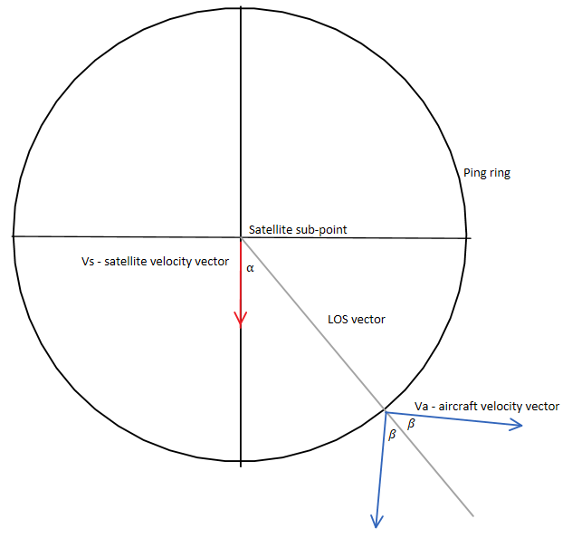
So the LOS speed between the satellite and the aircraft along the LOS vector is as follows:
-
\(LOS\)
- Line Of Sight
-
\(EA\)
- Elevation Angle between the aircraft and the satellite \(V_s\)
- Satellite’s velocity vector
-
\(V_a\)
- Aircraft’s velocity vector
-
\(\alpha\)
- Bearing angle from the satellite to the aircraft’s position
-
\(\beta\)
- Angle between the aircraft’s velocity vector and the \(LOS\)
If we assume a particular position for the aircraft on the ping ring and a particular ground speed for
the aircraft then given we have the LOS speed from the BFO Doppler data we can solve for
\(\beta.\)
Couple of assumptions/simplifications.
- Assuming that Vx and Vy are 0 for the satellite and only using the Vz component.
- Assuming that Vx is 0 for the aircraft
At 00:11UTC at the time of the last ping the satellite’s velocity components were:
$$V_z = -82.1m/s$$
$$V_x = 1.5m/s$$
$$V_y = -1.5m/s$$
Using the following data from Duncan Steel - duncansteel.com.
| Time (UTC) | Elevation Angle | Ping Radius (nm) | LOS Speed DS (kt) | LOS Speed POL (kt) | Satellite Z (nm) | Satellite Vz (kt) |
|---|---|---|---|---|---|---|
| 18:29 | 53.53 | 1880 | 39.77 | 76.24 | 623.87 | 49.12 |
| 19:40 | 55.80 | 1760 | 39.14 | 4.97 | 651.30 | -3.22 |
| 20:40 | 54.98 | 1806 | 65.80 | 57.02 | 625.88 | -47.42 |
| 21:40 | 52.01 | 1965 | 79.85 | 118.34 | 557.62 | -88.38 |
| 22:40 | 47.54 | 2206 | 100.64 | 175.49 | 451.20 | -123.31 |
| 00:11 | 39.33 | 2652 | 125.35 | 250.43 | 233.91 | -159.58 |
- DS - Duncan Steel & Mike Exner BFO analysis
- POL - Polynomial fit of BFO data -
\(BFO = 0.3673 * |LOS\ vel\ in\ km/hr| + 94.975\)
I’ve written a Python script that uses the formula above and the data above to iterate over a number
of sample aircraft positions along the 00:11UTC ping ring by iterating over
\(\alpha\)
from 1 degree to 89 degrees.
An assumed aircraft ground speed is entered as a parameter and for each sample position along the ping arc
the script calculates
\(\beta\)
and derives 2 possible ground tracks for the aircraft at the sample position to
match the known LOS speed from the BFO Doppler data.
Given the ground tracks calculated and the supplied aircraft ground speed and the time between this ping and the previous ping the script calculates the aircraft’s position at the time of the previous ping assuming a constant ground speed and constant ground track.
If the computed aircraft position at time of the previous ping is within 2% of the previous ping ring then the aircraft’s position on the current ping ring and it’s calculated position on the previous ping ring are plotted with a line joining them.
The script then continues recursively using the points that are within 2% of the previous ping ring to compute
\(\beta\)
for each of them based on the LOS speed for this ping ring and working backwards to the
previous ping ring.
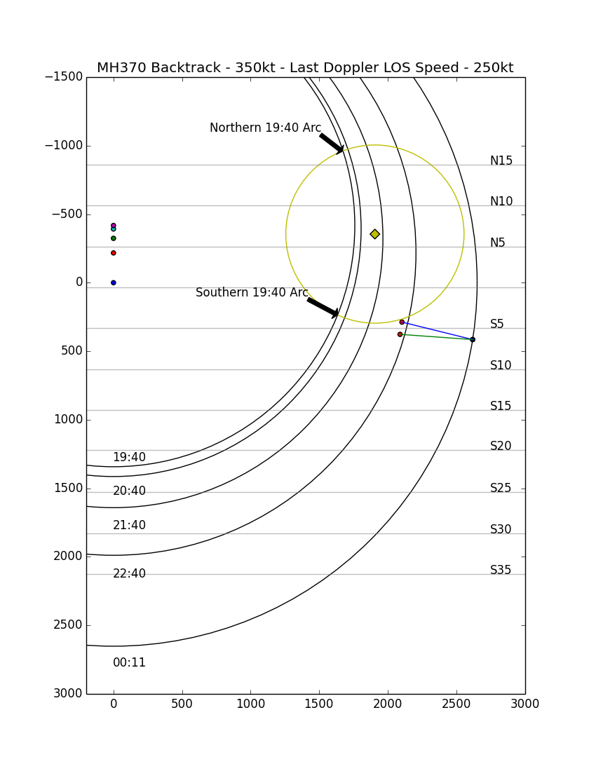
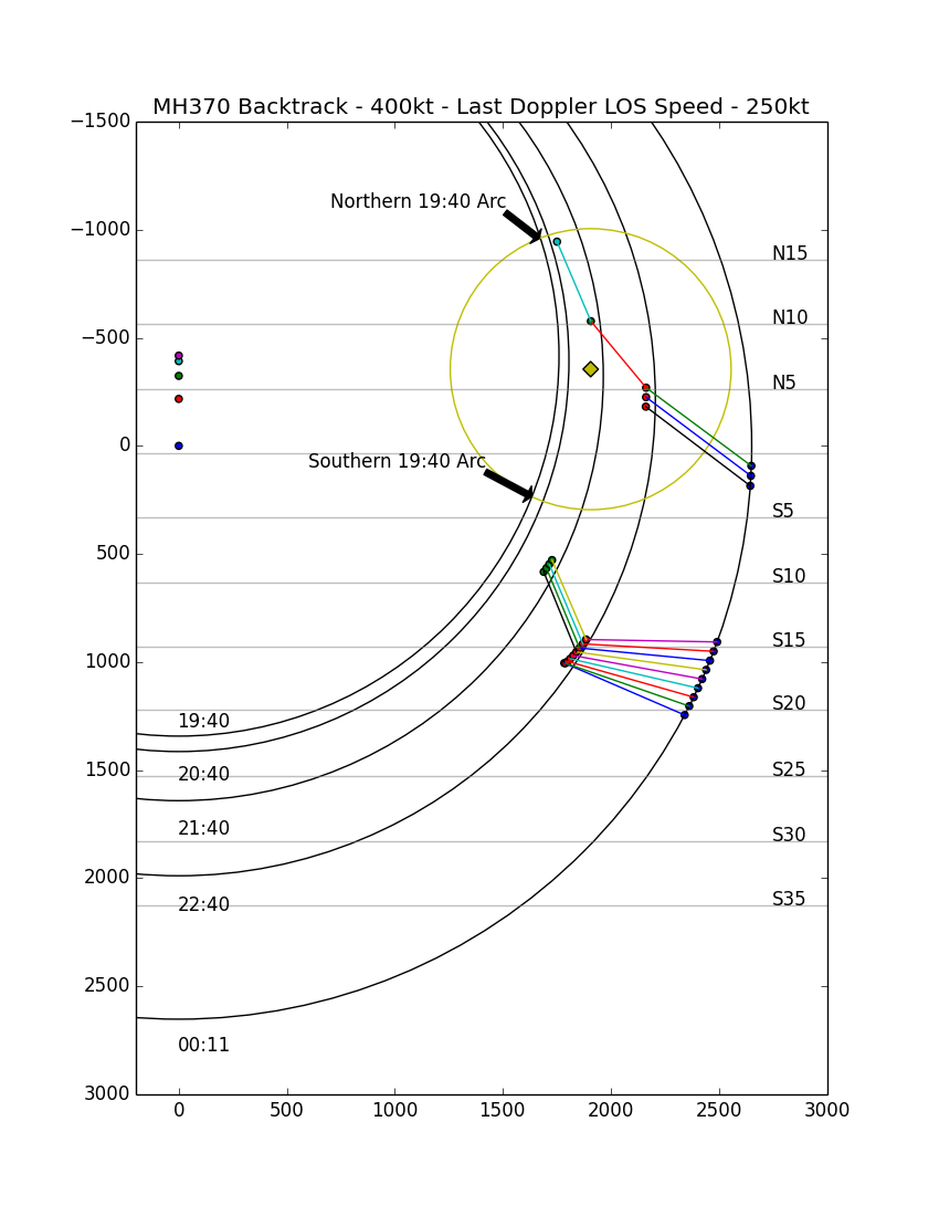
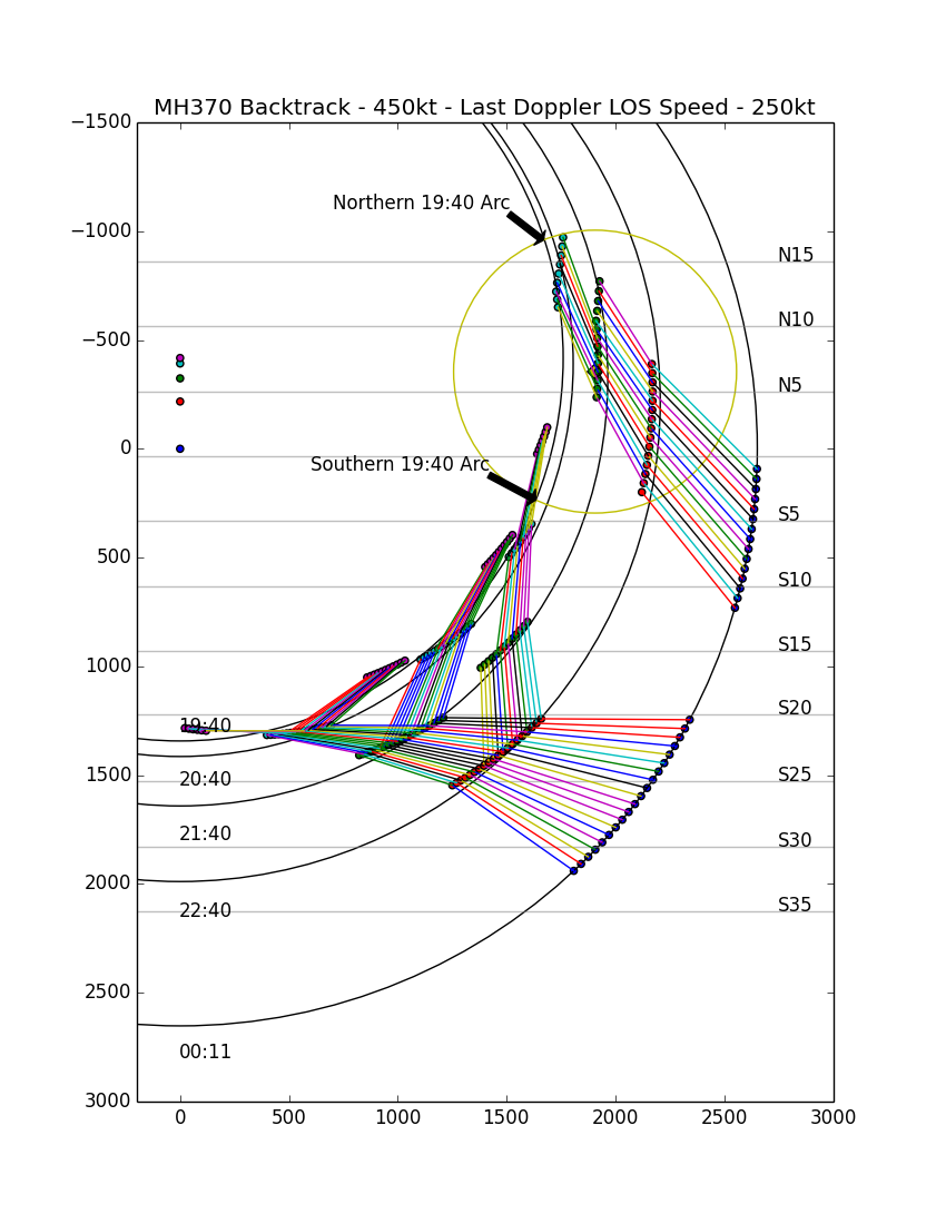
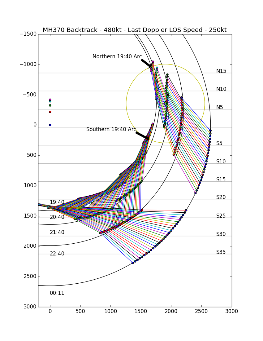
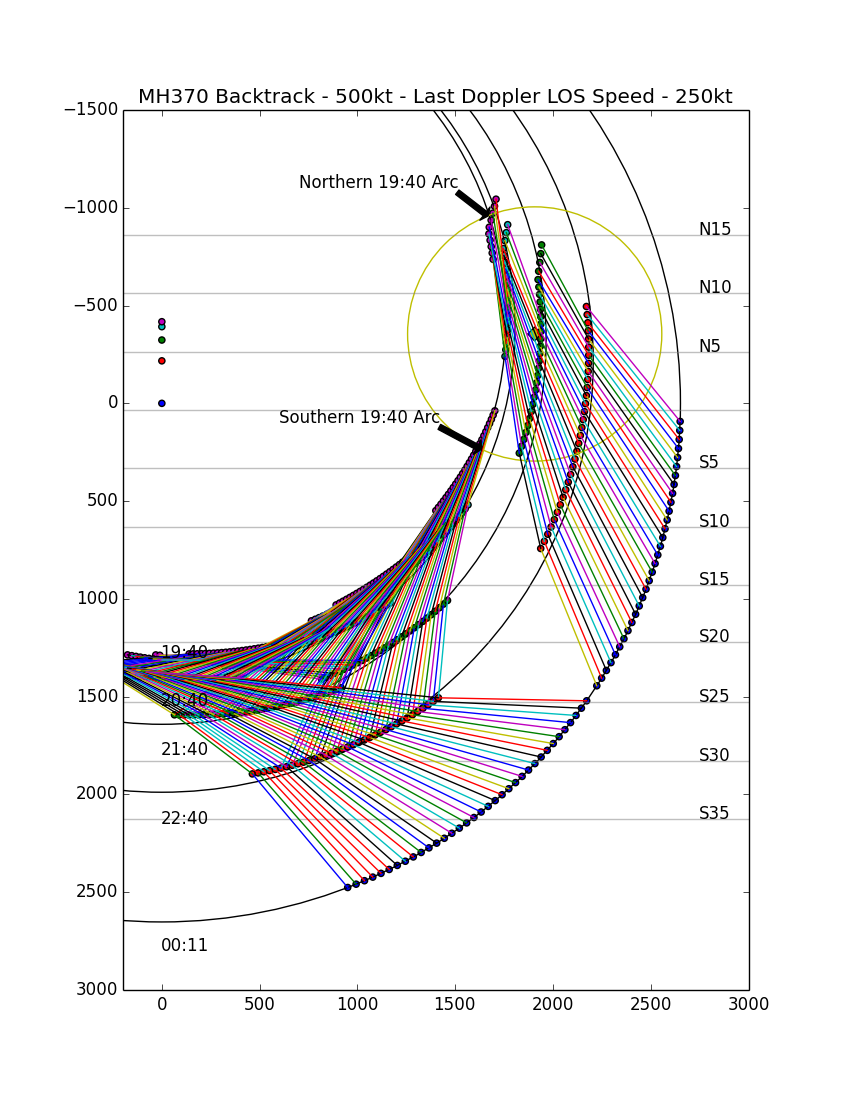
For a given aircraft ground speed the resulting plot shows the range of possible aircraft positions on the 00:11UTC ping ring and ground track that match the BFO LOS speed and which track back to intersecting the previous ping ring at the correct time.
The idea was to get a feel for the range of possible locations on the 00:11UTC ping ring for a given aircraft ground speed that also matches the BFO LOS speed data at that time and to see how many of those tracks track back to the 19:40UTC ping ring.
The plots also include the last known location for the aircraft at 18:22UTC from the Malaysian military radar, indicated as a yellow diamond. I’ve then assumed a maximum ground speed of 500kts from this time and location for 78 minutes until the 19:40UTC ping and rendered the maximum range that could be covered (650nm) in this time as the yellow circle.
The intersection of this circle with the 19:40UTC ping ring places a maximum northern and southern limit to where the aircraft could be at 19:40UTC along this arc.
When I initially started thinking about writing this program I was only aware of the BFO LOS speeds that Duncan Steele and Mike Exner had calculated. However none of Duncan’s routes that he tried in STK could match the LOS speeds that had been calculated from the BFO data. The routes did match the relevant ping ring times but there was no match for the BFO Doppler data.
Subsequently I became aware from a comment on Duncan Steele’s blog posting for an alternative set of BFO derived LOS speeds. I’ve listed both in the table of data that I’m using above and the Python script takes the LOS speed for the ping ring as an input parameter.
In running the script however there are no matches for any airspeeds tested between 350kts and 500kts that produce any matches using Duncan Steele and Mike Exner’s BFO derived LOS speeds, so in all the plots below I’ve only used the BFO derived LOS speeds from the polynomial fit approach.
Source code for the Python program - MH370Backtrack.py
Plots for 350kt, 400kt, 450kt, 480kt and 500kt.